Graph Mode Design Document

Overview

xLLM’s Graph Mode supports multiple graph execution backends. Its goal is to turn the original Host-driven stream of fine-grained kernel launches into a capture-then-replay execution flow in inference serving, thereby reducing Host scheduling overhead, reducing device-side bubbles, and improving throughput and latency stability.

This document is intended for developers who need to understand the implementation principles and key design choices. It focuses on:

• the basic Graph Mode mechanism and how xLLM applies it
• dynamic dimension parameterization
• Piecewise Graph
• a multi-shape reusable memory pool, including input tensor reuse

This document focuses on the unified Graph Mode design in xLLM and does not expand on backend-specific platform differences.

The design goals of this document are:

• provide a unified Graph Mode abstraction across xLLM backends
• explain the three key designs: dynamic dimension parameterization, Piecewise Graph, and multi-shape memory reuse
• clarify what problem each design solves, what assumptions it depends on, and where its boundary lies

The non-goals of this document are:

• full adaptation details for every operator or every model
• replacing feature documentation for flags and usage examples

Related design documents:

• for a recommendation-oriented case study that focuses on fixed scheduling, multi-step execution, and custom operators, see: Generative Recommendation Design Document

1. Graph Mode Fundamentals

1.1 Capture / Replay Basics

In traditional eager execution, one forward pass launches many kernels, memory copies, and synchronization operations from the Host. For decode-like workloads, where each step is small but requests are frequent, Host scheduling overhead becomes significant and device-side bubbles become more visible.

The core idea of Graph Mode is:

1. Capture: when a shape bucket is seen for the first time, run one forward pass on a dedicated stream and record the kernel launches, memory operations, and dependencies into a graph.
2. Replay: for later requests that hit the same bucket, replay the recorded graph instead of launching kernels one by one from the Host.

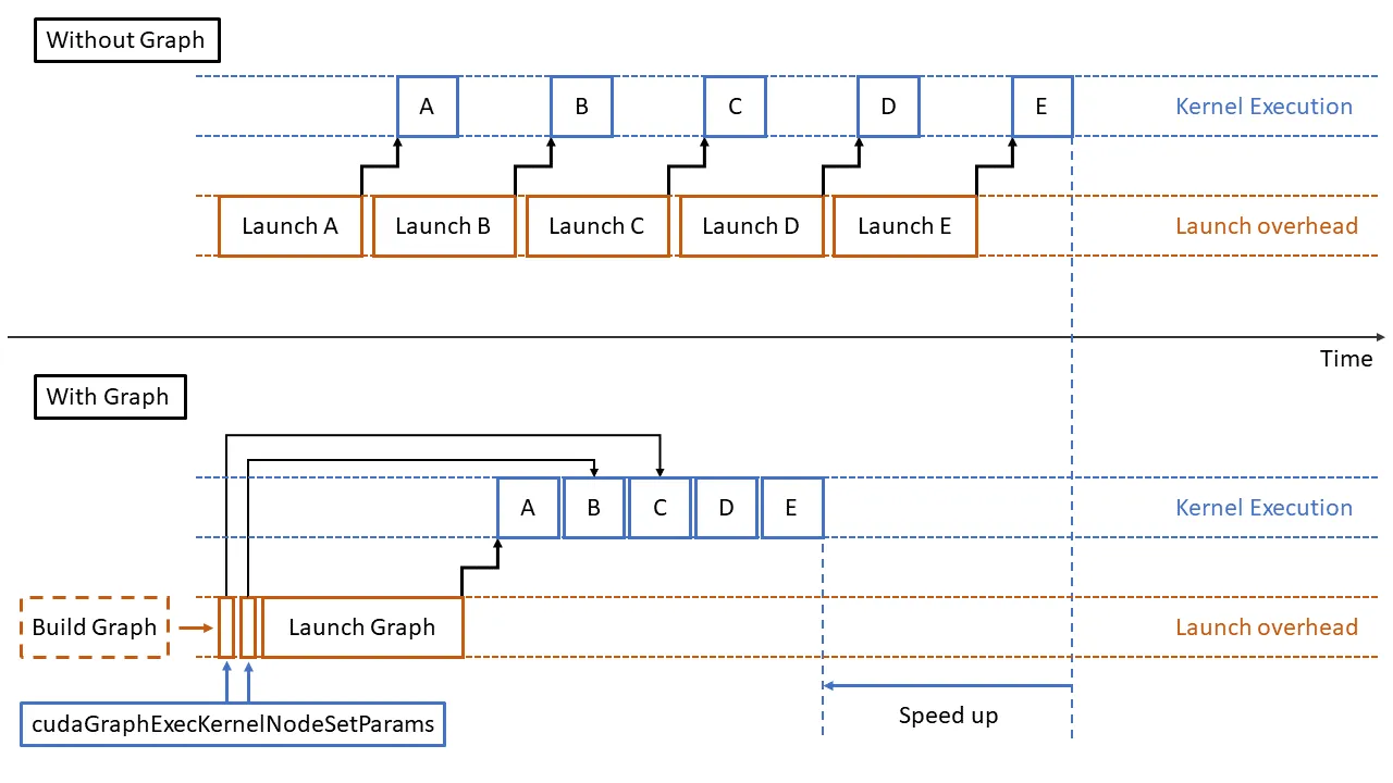
This mechanism usually requires:

• Stable execution path
  • graph capture records one concrete execution path; once capture completes, the control flow, launch shape, and dependencies on that path are fixed
  • therefore, the capture path cannot switch to a different dynamic branch during replay
• Stable addresses for key tensors
  • key tensor addresses written into the graph during capture must still be valid at replay time
• Stable operator behavior and result semantics
  • replay correctness depends on operators along the path being Graph Mode compatible and not changing semantics because of runtime condition changes

1.2 xLLM GraphMode Runtime Foundations

Starting from the three basic requirements in 1.1, the first two are mainly handled by the xLLM runtime: turning dynamic requests into execution units that can be replayed stably, and ensuring replay still accesses the fixed addresses recorded during capture. For that reason, xLLM introduces a unified Graph Executor in Graph Mode to centralize bucketing, persistent buffers, graph cache management, and the capture / replay lifecycle.

xLLM’s runtime-side foundation work mainly includes:

• Graph selection and execution scheduling around execution-path stability
  • requests must first be grouped into buckets by num_tokens or a nearby shape
  • graph cache is maintained per bucket: replay directly on a hit, otherwise capture first and cache the graph
  • use full graphs for paths that are fully capturable, and switch to Piecewise Graph when part of the path breaks graph capture
• Persistent buffer and graph-instance management around address stability
  • dynamic inputs such as tokens, positions, seq_lens, and block_tables cannot be reallocated to arbitrary new addresses before replay; xLLM must write them into persistent buffers first and then update content at fixed addresses
  • tensors allocated temporarily during model graph construction also need to be retained with the corresponding graph instance instead of being reclaimed when their local scope ends
  • when the shared memory pool is enabled, captures of different shapes can reuse the same underlying physical memory, while the virtual addresses seen by the graph still remain stable
• A unified Graph Executor abstraction
  • capture, cache, replay, graph-instance management, and backend abstraction all need to be handled centrally by the runtime
  • the point of this layer is to pull Graph Mode runtime orchestration out of model code rather than scattering it across layers or operators

In concrete execution, the Graph Executor runtime flow can be summarized as:

1. Bucket the request: group the request into a bucket by num_tokens or a nearby shape.
2. Prepare inputs: write tokens, positions, seq_lens, and block tables into persistent buffers, and update runtime metadata such as attn_metadata and plan_info.
3. Choose capture or replay: replay directly if the bucket already has a cached graph; otherwise capture, cache, and then enter the replay path.
4. Execute the graph: run a full graph or a piecewise graph depending on the scenario.

The third requirement in 1.1, “stable operator behavior and result semantics”, falls more on model-side and operator-side adaptation, which is covered in 1.3.

1.3 Model Adaptation Required for Graph Mode

After the xLLM runtime takes care of bucketing, buffers, and graph-instance management, the model side still needs to satisfy the third requirement from 1.1: operator behavior and result semantics must remain stable across capture / replay and must not break because of host participation, dispatch changes, or launch-shape changes.

The required model adaptations mainly include:

• Remove operations that are not capture-safe
  • General requirement: the capture path must not contain operations that trigger host-side decisions, implicit host-device synchronization, or extra control-flow changes, such as stream synchronization, logic branches driven by host tensors, or implicit host-device interactions
  • Typical example 1: operators may depend on host tensor contents to decide task partitioning or execution mode. For example, ATB PA and MLA in Ascend CANN commercial 8.3 can choose different task layouts based on host-side kv_seq_lens and q_seq_lens
  • Typical example 2: a host scalar participates in tensor computation, or the host directly reads tensor data, for example:

Tensor a;
Tensor b = a * 0.5;  // the scalar is implicitly transferred to the tensor's device, causing a synchronized H2D

torch::Tensor max_of_seq = torch::max(input_params.kv_seq_lens);
max_seq_len_ = std::max(max_of_seq.item<int>(), max_seq_len_);  // host reads tensor data

• Adapt operators
  • General requirement: the kernel execution path must remain stable for the same input shape. For one input shape, graph execution should choose the same kernel every time, without mixing prefill, chunked prefill, and decode behavior. At the same time, grid_dim, block_dim, task count, workspace shape, and tiling content must also remain stable
  • Typical example: in Ascend CANN commercial 8.3, ATB PA may decide at runtime whether to enable flash-decoding long-sequence mode based on sequence length and batch size. The long-sequence and short-sequence modes use different tiling keys, and the actual dispatched kernel_name is also different. This kind of behavior, where the same business path triggers different kernels under different runtime conditions, must be converged before entering Graph Mode

2. Dynamic Dimension Parameterization

2.1 Problem

Graph capture records a fixed kernel sequence and the launch parameters of every kernel. At replay time, the runtime can only repeat that recorded launch shape. It cannot re-decide grid_dim, block_dim, task count, or the tiling path inside the same graph.

As a result, not every dynamic request dimension can continue to vary once the request enters Graph Mode. For attention, the real dynamic factors usually include more than num_tokens: they also include batch_size, q_seq_lens, kv_seq_lens, and block_tables_size. If these dimensions further affect task partitioning, workspace layout, tiling_params, or kernel path, replay may reuse the stale capture-time configuration and become incorrect.

The core question of this chapter is therefore: which dynamic information can still be updated after the graph has been selected, and which dimensions must instead be handled by finer-grained bucketing or by building another graph.

2.2 Solution

The goal of dynamic dimension parameterization is not to make one graph accept arbitrary num_tokens. Instead, once the graph has already been selected by bucket_num_tokens, the goal is to let the same bucket safely cover more real dynamic requests.

2.2.1 Parameterization Boundary

Whether a dimension can still vary at replay time does not depend on whether it is dynamic in the request. It depends on whether that dimension has already been folded into the execution shape during capture.

Dynamic factors can be divided into two categories:

1. Dimensions that determine graph shape

   • once a dimension enters grid_dim, block_dim, task count, workspace layout, tiling key, or tiling_params, it becomes part of the capture result
   • after that, it usually cannot be changed inside the same graph

2. Dimensions that can still be updated after graph selection

   • such as batch_size, q_seq_lens, kv_seq_lens, block_tables, new_cache_slots, and plan_info
   • they are suitable parameterization targets only if they do not further rewrite execution shape

A simplified norm-kernel example is:

int grid_dim = num_tokens;
NormKernel<<<grid_dim, block_dim>>>(x, y, ...);

Here, grid_dim and block_dim are both launch parameters. Once num_tokens participates in launch configuration, it becomes part of graph shape; after capture, replay can no longer change grid_dim = 128 into grid_dim = 256 within the same graph.

So the boundary is straightforward: any dynamic factor that changes launch shape, workspace, or tiling path should not be handled only by updating parameters before replay.

2.2.2 How xLLM Handles It

xLLM handles this in two layers.

The first layer handles num_tokens: xLLM uses bucketing and padding to normalize the raw request into a fixed bucket_num_tokens, and then selects the graph accordingly.

The second layer handles the remaining dynamic information inside that bucket: adapt operators that depend on host tensors, host planning, or host-side tiling so that request-varying information is stored in device-side persistent buffers, or otherwise externalized into data that can be refreshed before replay, instead of letting replay stay bound to the old host-side planning result from capture.

Take NPU attention as an example. A common pre-adaptation problem is that q_seq_lens and kv_seq_lens first participate in host-side planning, which produces task, workspace, or tiling-related data before launching the kernel:

// Host side
auto plan_info = PlanAttention(q_seq_lens_host, kv_seq_lens_host, ...);
WritePlanToWorkspace(attention_workspace, plan_info);

AttentionKernel<<<grid_dim, block_dim>>>(
    q, k, v, out,
    attention_workspace,
    tiling_params);

In this kind of implementation, graph replay does not automatically redo planning, so it can only repeat the launch shape and workspace layout from capture time. The adapted direction is to write request-varying information such as q_seq_lens, kv_seq_lens, block_tables_size, and plan_info into device-side persistent buffers under a fixed launch shape, and let the kernel read them directly. For example, a parameterized kv_seq_lens path may look like:

struct AttentionLaunchArgs {
  void* q;
  void* k;
  void* v;
  void* out;
  int32_t batch_size;
  int32_t* kv_seq_lens;   // device buffer
  void* attention_workspace;
  void* tiling_params;
};

LaunchAttentionKernel(args);

If a dynamic factor changes task count, array length, workspace shape, or tiling path as soon as it varies, xLLM does not force it into “parameterization updates”. Instead, it uses one of two approaches:

1. expand the bucketing dimensions and include those factors in the graph-selection key, for example a combination of num_tokens and num_comm_tokens
2. keep that dynamic-shape-sensitive part outside the full graph and handle it with Piecewise Graph

2.3 Result

Dynamic dimension parameterization directly brings the following result: one num_tokens bucket can safely cover more real requests, and under a stable execution shape, operators such as attention can still see the correct dynamic information at replay time, including batch_size, seq_lens, block_tables_size, and plan_info.

One thing to keep in mind is that parameterization does not eliminate bucketing. The dynamic nature of num_tokens is still mainly absorbed by graph selection; if a bucket still contains other factors that rewrite tiling keys, task count, communication scale, or kernel path, those factors must still enter the bucketing key or move to Piecewise Graph. Communication-heavy scenarios are a typical example. In Attention DP + MoE EP, communication scale may depend on the maximum DP data size rather than strictly matching local num_tokens on one device.

3. Piecewise Graph

3.1 Problem

In prefill and chunked prefill scenarios, the full forward path is usually more complex than decode. Some operators may:

• fail to be captured stably
• be highly sensitive to dynamic metadata
• rely on extra runtime preparation during capture

If the requirement is that the entire path must be capturable as one full graph, Graph Mode coverage becomes very limited. Once one critical operator breaks graph capture, the whole path loses graph execution.

3.2 Solution

3.2.1 Underlying Logic

One common question in implementation is: why can decode use a full graph while chunked prefill usually needs Piecewise Graph?

The key difference is attention.

Under current decode semantics, one step usually means one generated token per sequence, so num_tokens and batch_size are almost one-to-one. For attention, that means:

• when num_tokens grows, batch_size grows with it
• the pattern of q_seq_lens stays relatively stable
• task partitioning, workspace requirements, and launch arguments can mostly be bucketed together with num_tokens

Therefore, when building buckets by num_tokens, decode satisfies the reuse conditions for a full graph.

In chunked prefill, however, num_tokens and batch_size are no longer tied together. The same num_tokens may correspond to very different request combinations, for example:

• num_tokens = 128, batch_size = 2, q_seq_lens = [64, 64]
• num_tokens = 128, batch_size = 4, q_seq_lens = [32, 32, 32, 32]
• num_tokens = 128, batch_size = 8, q_seq_lens = [16, 16, 16, 16, 16, 16, 16, 16]

For attention, these requests share the same num_tokens but they are not the same shape. Attention task partitioning, local indexing, the lengths of q_seq_lens and kv_seq_lens, and the corresponding plan_info all directly depend on batch_size. If the system reuses a previously captured graph only by num_tokens, then replay may keep using the old batch partitioning and old task partitioning from capture, which can make the result incorrect.

batch_size is hard to parameterize here because it changes more than just one scalar value. It changes the structure of the launch arguments themselves:

• the lengths of q_seq_lens and kv_seq_lens change
• the task count and task boundaries of attention change
• plan_info and workspace layout change
• the indexing and partition logic inside the kernel change

In other words, in chunked prefill, batch_size is not a dimension that can be handled by updating a few parameters. It changes the execution shape of the attention part itself. Unless num_tokens × batch_size, or even more fine-grained seq_lens combinations, are added into bucketing, selecting graphs only by num_tokens is not safe.

That is why the current design is better suited to:

• decode: attention can be captured together with the full graph
• chunked prefill: attention stays outside the graph while the more stable surrounding parts enter Piecewise Graph

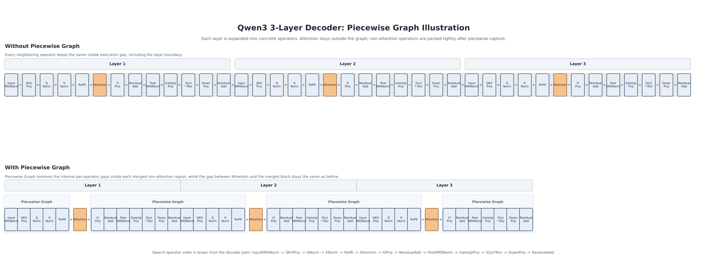
3.2.2 Core Idea

The goal of Piecewise Graph is not to force full-graph capture. It is to split one full execution path into several pieces:

• graph-friendly parts: captured into subgraphs
• parts that are not suitable for graph capture: kept in eager mode

At replay time, those pieces are executed in the same order recorded during capture.

This preserves as much Graph Mode benefit as possible even when full-graph capture is not feasible.

The following diagram uses a three-layer Qwen3 decoder as an example. Attention stays as an independent runner, while the non-attention operators between attention calls are packed as tightly as possible into continuous graph pieces.

3.2.3 How xLLM Implements It

In xLLM, Piecewise Graph is mainly used for prefill-like scenarios and is controlled by enable_prefill_piecewise_graph.

Its core implementation is:

1. use PiecewiseGraphs to maintain the replay instruction sequence
2. store capturable segments as graph objects
3. record non-graph attention segments as runners through AttentionRunner
4. replay in the original order as graph -> runner -> graph -> ...

The key point is how attention is handled:

• during piecewise capture, attention temporarily ends the current graph capture
• attention itself is not executed during capture; instead, the tensors, workspace, and parameters required for attention are recorded
• at replay time, attention runs with the latest plan_info, q_cu_seq_lens, and kv_cu_seq_lens

The direct reason is that, in chunked prefill, attention has dynamic dimensions beyond num_tokens, while current graph bucketing is mainly organized by num_tokens. Keeping attention outside the graph avoids replay errors where the graph hits by num_tokens, but batch_size and seq_lens have already changed.

So the essence of Piecewise Graph is not to support all dynamic attention logic inside the graph. It is to:

• put the stably capturable parts into graphs
• keep the more dynamic-shape-sensitive attention as a separate execution unit
• preserve the original execution order through one unified instruction sequence

3.3 Result

The results and boundaries of this design are reflected in the following aspects.

3.3.1 Applicable Scenarios

• prefill
• chunked prefill
• scenarios with local graph breaks where graph execution benefit is still desired for the overall path

3.3.2 Benefits

• more flexible than all-or-nothing full-graph capture
• significantly expands Graph Mode coverage
• fits model structures where attention is highly dynamic while parts such as MLP remain relatively stable

3.3.3 Limitations

• currently focused mainly on prefill-like paths
• replay depends on correctly updated attn_metadata.plan_info

4. Multi-Shape Reusable Memory Pool

4.1 Problem

In multi-shape scenarios, Graph Mode faces two problems at the same time:

1. capture-time memory grows linearly with the number of shapes

   • each new shape entering capture usually gets its own independent memory buffer pool
   • because Graph Mode requires stable addresses between capture and replay, these buffers often cannot be released in time
   • memory usage grows from the expected max(shape) to sum(shape)

2. input-side memory is also repeatedly duplicated

   • if each shape keeps its own tokens, positions, seq_lens, block_tables, and related tensors
   • then even if the graph itself can be reused, input-side memory still accumulates by shape

So the reusable memory pool is not just about saving memory. It is about supporting dynamic new shapes while making memory usage converge from sum(shape) to max(shape).

The concrete goals include:

1. capture-time memory reuse: different graphs share the same underlying physical memory
2. input-side memory reuse: replays of different shapes share one set of persistent input buffers
3. no address conflicts: every captured graph still keeps its own stable virtual address view
4. on-demand support for new shapes: a new shape can still be captured without invalidating existing graphs
5. no extra replay overhead: most reuse happens during capture and input preparation, while replay stays as unchanged as possible

4.1.1 Root Cause

• on the CUDA path, the allocator typically allocates an independent memory buffer pool for every graph capture
• Graph Mode then requires stable addresses between capture and replay, so buffers from old shapes cannot be reclaimed like ordinary eager temporary memory
• as more shapes enter capture, memory usage grows from the expected max(shape) to sum(shape)

4.1.2 Constraints

• under the current assumption, graphs of different shapes do not replay simultaneously
• dynamically appearing new shapes must still be supported through on-demand capture
• existing graph caches should not be torn down just because a new shape appears
• replay should not become more complex because of memory reuse

4.1.3 Failed Approach and Technical Challenge

A more direct idea is to reset the allocation pointer before each capture so that different shapes reuse the same virtual address space.

But this is not safe in practice. Allocators usually track allocated blocks by address. If a new capture reuses an old address, it may overwrite the previous address record. Then, when tensors belonging to an old graph are later destructed or freed, the address record may already be gone, which can trigger errors such as invalid device pointer.

This reveals the real challenge: what Graph Mode truly needs to keep stable is the address view seen by each graph, while what really needs to be reused is the underlying physical memory. So the problem is not just memory saving. It is how to satisfy all of the following at the same time:

• the virtual address spaces of captured graphs do not conflict
• the underlying physical memory can still be shared across shapes
• adding a new shape into capture does not break replayability of already captured graphs

4.2 Solution

The core idea is not to let different shapes share one virtual address range. Instead, it is to let them share one set of physical memory while each captured graph keeps its own virtual address view.

The reason is simple: if different shapes are forced to reuse the same virtual address space, allocator address tracking will conflict, and old graphs may no longer find their original address records when they are released or destroyed. In other words, the thing that must be reused is the underlying physical memory, not the virtual address seen by the graph itself.

To show why xLLM chooses “shared physical memory + independent virtual address spaces”, the common solutions can be compared as follows:

Solution	Memory reuse mechanism	Physical memory outcome	Address-conflict risk / mitigation	Main limitation
vLLM	Shared graph memory pool + capture larger shapes first	may still approach sum(shape)	relies on a shared memory pool and free-block management, usually without explicit address conflicts	reuse efficiency depends on capture order and allocator behavior
SGLang	Global graph memory pool + capture larger shapes first	may still approach sum(shape)	relies on global pool or graph-private pool management to avoid conflicts	memory still grows when there are many distinct shapes
xLLM	Map multiple virtual address spaces to one set of physical memory	converges to max(shape)	every graph keeps an independent address view, avoiding address-record conflicts at the root	depends on VMM and allocator integration support from the runtime

xLLM does not reuse the same virtual address space. Instead, each graph keeps its own address view, while the truly shareable part is pushed down into underlying physical memory.

4.2.1 Multi-Shape Input Tensor Reuse

xLLM first solves repeated input-side memory usage. Instead of allocating independent input tensors for each shape, it pre-allocates one set of persistent buffers for the maximum shape and lets different shapes share them.

These buffers usually include:

• tokens
• positions
• q_seq_lens
• kv_seq_lens
• block_tables
• new_cache_slots
• hidden_states

Replay-time handling is straightforward:

1. write the actual input of the current request into the prefix of the buffer
2. zero-fill padding regions when needed
3. construct slice views for the actual shape

As a result, input-side memory no longer accumulates by shape and stays at one max(shape) allocation.

4.2.2 Capture-Time Memory Reuse

After solving input duplication, xLLM still needs to solve the memory accumulation caused by graph capture itself.

The core design is:

• every capture uses a new virtual address space
• different virtual address spaces map to the same physical memory

This satisfies two requirements at once:

1. stable addresses from the graph’s point of view: each captured graph sees its own fixed virtual addresses
2. only one physical-memory footprint: the underlying physical memory grows by the maximum demand instead of accumulating by shape

Compared with reusing one virtual address range, this design avoids address-tracking conflicts and therefore works better with existing allocator mechanisms.

This design relies on a unified virtual memory management capability, including:

• reserving a new virtual address space
• creating or expanding underlying physical memory
• mapping the same physical memory into multiple virtual address spaces
• performing unmap, address-space release, and access-permission operations when needed

The key property is that the same physical memory can be mapped into multiple virtual address spaces. That is exactly what makes “different graphs have independent addresses while still sharing the same physical memory” possible.

4.2.2.1 Address Mapping Relation

The core mapping relation for capture-time memory reuse is shown below:

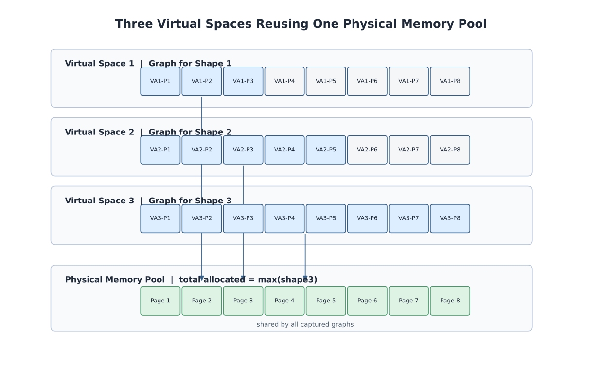
This diagram shows that, as the shape grows, each new capture switches to a new virtual address space, while all three virtual spaces reuse the same physical memory pool. Different shapes only use different portions of that pool, and the total physical memory converges to max(shape).

4.3 Results

4.3.1 Memory Efficiency Metrics

Metric	Without memory reuse	With memory reuse
Physical memory size	sum(shape)	max(shape) ✅
Virtual memory	multiple copies	multiple copies
Stability	address-conflict risk	stable ✅

The key change is that physical memory converges to max(shape), while virtual address space still grows with the number of captured shapes.

4.3.2 Performance Impact

• capture stage: switching virtual address spaces and extending mappings introduces extra overhead
• replay stage: no extra graph execution overhead, and behavior is essentially the same as normal Graph Mode replay
• input preparation stage: one extra write into persistent buffers plus slice-view construction, which is still typically cheaper than repeated allocation

4.3.3 Virtual Address Space Overhead

One cost of this design is that virtual address space grows as more shapes are captured. But this growth is address-space usage, not physical memory usage.

On 64-bit systems, virtual address space is usually much larger than single-device memory capacity, so it is typically not the primary bottleneck for this kind of graph capture scenario. In other words, this design uses abundant address space to bring physical memory down from sum(shape) to max(shape).

4.3.4 Result Validation

• captures of different shapes can share the same underlying physical memory
• every capture still keeps an independent virtual address space instead of reusing the same address view
• address-conflict issues are no longer exposed through the failed “reuse one virtual address space” path
• memory usage converges from sum(shape) to max(shape)

4.3.5 Practical Effects

• in multi-shape scenarios, memory behavior changes from “grows linearly with captures” to “physical memory converges to the maximum shape”
• graph reuse becomes more stable because direct reuse of one virtual address space is avoided
• the design supports on-demand capture for new shapes without tearing down existing graph caches
• replay stays unchanged or nearly unchanged, while most added complexity is concentrated in capture and input preparation

4.3.6 Assumptions and Boundaries

• virtual address space still grows with the number of captured shapes, even though physical memory only grows with the maximum demand
• the design depends on runtime support for virtual address management, physical memory mapping, and allocator integration
• it currently assumes that graphs of different shapes do not replay simultaneously; that assumption is what makes physical memory sharing safe
• the current implementation still keeps physical memory and virtual spaces for the full lifecycle instead of doing fine-grained dynamic release

5. References

• ACLGraph Capture / Replay mechanism
• CudaGraph capture mechanism
• vLLM graph execution reference
• SGLang graph execution reference